How to automatically transform a crosstab table to a flat list in Excel without VBA macros.
XLTools Automation tool allows you to automate tasks in Excel by creating automation commands in a table, without having to create VBA macros.
This tutorial will take you through the setup of the UnpivotTable automation command. Use it when you need to transform a crosstab table to a flat list. This command is especially useful when you need to process the resulting flat list later on.

For non-recurring tasks, use the standard Unpivot Table tool on XLTools ribbon.
Before you begin, add the Automation tool to Excel
Automation is one of the 20+ features within XLTools Add-in for Excel. Works in Excel 2024, 2019, 2016, 2013, 2010, and Microsoft 365.

Step-by-step example: how to use the UnpivotTable command
Say, your pricelist for different product categories is arranged as a crosstab table. If you want to use this data in some further calculations, first, you need to transform the crosstab table to a flat list. And every time you get an updated pricelist you have to do the same again and again.
When you automate this process with the UnpivotTable command, you can transform the crosstab table in a button click. Follow the steps below to execute the command yourself.
Feel free to download the sample file used in this tutorial.
1. Insert the UnpivotTable command
- Let's take a look at the Excel spreadsheet and data you want to unpivot. In our example, the spreadsheet contains the worksheet "Pricelist".
- Add a new worksheet → Name it, for example, "AUTO". This worksheet will hold automation commands.Tip:it's best to keep automation commands on a separate worksheet, not to interfere with data.
- Select a starting cell where to place the command, e.g. A1.
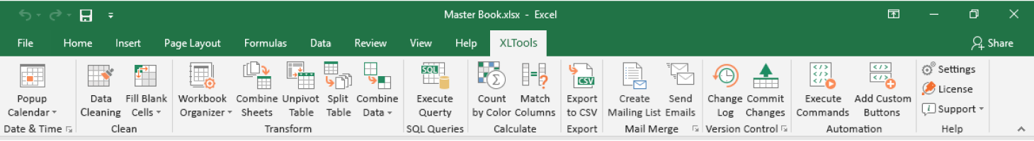
- Open XLTools tab → In the Automation group, open the drop-down list → Select UnpivotTable.
- See the table with the automation command is now added on the worksheet.

2. Specify parameters and define how to unpivot table
Once you've inserted the UnpivotTable command, specify its parameters. This automation table defines how to unpivot the Excel table and convert it to a flat list.
| XLTools.UnpivotTable | |
|---|---|
| Range: | Pricelist!A:E |
| SkipEmptyValues: | TRUE |
| SkipDuplicates: | FALSE |
| HeadersOnly: | FALSE |
| HeaderColumnsCount: | 1 |
| HeaderRowsCount: | 1 |
| ValuesFilter: | |
| LeaveMaxValueInRow: | TRUE |
| FixedColumns: | |
| FillMergedCellsWithDuplicates: | FALSE |
| PreserveFormat: | FALSE |
| PreserveHeaders: | TRUE |
| SplitValueBy: | |
| KeepWorkbookOpen: | TRUE |
| ApplyTableName: | Flatlist |
| TableSortRange: | |
| OutputTo: | NewSheet[Result] |
What each line in this command reads:
- Range: take the range A:E on the sheet Pricelist. This is the source range that we'll unpivot.
- SkipEmptyValues: choose TRUE to skip rows with empty values in the resulting flat list.
- SkipDuplicates: choose FALSE.
- HeadersOnly: choose FALSE.
- HeaderColumnsCount: type 1, as there is only one header column in the crosstab table (column A).
- HeaderRowsCount: type 1, as there is only one header row in the crosstab table (row 1).
- ValuesFilter: leave blank.
- LeaveMaxValueInRow: select TRUE.
- FixedColumns: leave blank.
- FillMergedCellsWithDuplicates: there are no merged cells in the source crosstab table, so let's choose FALSE.
- PreserveFormat: select FALSE, to get a flat list with plain formatting.
- PreserveHeaders: yes, let's keep the header from the source table and choose TRUE.
- SplitValueBy: leave blank.
- KeepWorkbookOpen: instruct to keep the workbook open.
- ApplyTableName: assign the name "Flatlist" to the resulting table.
- TableSortRange: leave blank.
- OutputTo: place the result on a new worksheet "Result" in the same workbook as the automation command.
See other available options to use in parameters.
3. Execute the command and review the resulting flat list
- Select the table of the automation command → In the Automation group, click Execute Commands.
- Review the resulting flat list:
- See that the flat list is generated on the new worksheet "Result"
- Unpivoted columns are automatically named "Category" and "Value"
Done! Now you can assign a custom button to this command.
If you need to run the command over and over again, add a custom button on the ribbon. So that next time you can execute the command in a click.
- In the Automation group, click Add Custom Buttons.
- Name the button, e.g. "Unpivot pricelist" → Specify the range of the UnpivotTable command → Click Save.
- Done! The custom button will appear on XLTools tab. Now every time you click this button, you will execute the command.
Note:
each time you execute the command, the newly generated worksheet will replace the previously generated worksheet. So before running the command next time, you can change its name in the OutputTo parameter.
Parameters and available options
When you create automation commands in Excel, this file with commands must be located in the same destination as the source data:
- Add automation commands in the same workbook as your source data. We recommend that you place the commands on a separate worksheet not to interfere with your data.
- Or, add automation commands in a separate workbook. Save this automation file in the same folder as the source data.
Below are all parameters and available attributes for the UnpivotTable command.
Tip:
select a cell and see a helpful tooltip. Some attributes also have a drop-down list of available options to choose from.
Range:
This parameter specifies which data range should be processed.
- Required parameter, cannot be blank
- If you refer to a source workbook, it can be open or closed
- The source workbook must be located in the same destination as the automation file
| Options | Meaning |
|---|---|
Sheet1!A1:B2 | Range A1:B2 on Sheet1 in the active workbook |
Sheet1!A:C | Entire A, B, C columns on Sheet1 in the active workbook |
Sheet1!1:3 | Entire 1, 2, 3 rows on Sheet1 in the active workbook |
Sheet1! | Entire Sheet1 in the active workbook |
Sheet1!@Table1 | Table1 on Sheet1 in the active workbook |
[Book1]Sheet1!A1:B2[Book1.xlsx]Sheet1!A1:B2 | Range A1:B2 on Sheet1 in the workbook Book1. Book1 must be located in the same destination as the automation file. |
C:\Documents\Workbook.xlsx | Specify the file path to the workbook |
Note:
Use standard rules of range referencing in Excel. If names of worksheets or workbooks contain spaces, enclose the name in single quotes, e.g. 'Orders April'!A1:H10, or '[All Orders]Orders April'!A1:H10. In order for automation commands to identify references, do not use spaces in the names of worksheets, workbooks, or tables.
SkipEmptyValues:
If your source table contains blank cells, you can instruct to skip empty values in the resulting flat list.
- Optional parameter, you can leave it blank or remove from the command altogether
| Options | Meaning |
|---|---|
| TRUE | If the source table contains blank cells, the corresponding rows in the resulting flat list will be skipped. Recommended if your source table has blank cells. |
| FALSE | If the source table contains blank cells, the corresponding rows in the resulting flat list will not be skipped. Use if your source table has no blank cells. |
| (blank) | Same as FALSE |
SkipDuplicates:
This parameter defines whether to skip duplicate rows in the resulting flat list.
- Optional parameter, you can leave it blank or remove from the command altogether
| Options | Meaning |
|---|---|
| TRUE | Skip duplicate rows |
| FALSE | Include all rows |
| (blank) | Same as FALSE |
HeadersOnly:
This parameter defines whether to return only headers without data.
- Optional parameter, you can leave it blank or remove from the command altogether
| Options | Meaning |
|---|---|
| TRUE | Return only headers |
| FALSE | Return headers and data |
| (blank) | Same as FALSE |
HeaderColumnsCount:
This parameter specifies how many header columns there are in the source table. In other words, the count of columns in the crosstab table header.
- Required parameter, cannot be blank
- Use a value between 1 and 100
| Options | Meaning |
|---|---|
| 1 | One header column |
| 2, 3 … | Two, three, or more header columns (multilevel headers) |
HeaderRowsCount:
This parameter specifies how many header rows there are in the source table. In other words, the count of rows in the crosstab table header.
- Required parameter, cannot be blank
- Use a value between 1 and 100
| Options | Meaning |
|---|---|
| 1 | One header row |
| 2, 3 … | Two, three, or more header rows (multilevel headers) |
ValuesFilter:
This parameter defines a filter for values in the resulting flat list.
- Optional parameter, you can leave it blank or remove from the command altogether
- The length of a text string in a cell cannot exceed 256 characters
LeaveMaxValueInRow:
This parameter defines whether to keep only the maximum value per row.
- Optional parameter, you can leave it blank or remove from the command altogether
| Options | Meaning |
|---|---|
| TRUE | Keep only the maximum value |
| FALSE | Keep all values |
| (blank) | Same as FALSE |
FixedColumns:
This parameter defines which columns should remain fixed (not unpivoted).
- Optional parameter, you can leave it blank or remove from the command altogether
FillMergedCellsWithDuplicates:
If your source table contains merged cells, you can instruct to duplicate values in merged cells in the corresponding positions in the resulting flat list.
- Optional parameter, you can leave it blank or remove from the command altogether
| Options | Meaning |
|---|---|
| TRUE | Values from merged cells in the source table will be duplicated in the resulting flat list. Recommended if your crosstab table has merged cells. |
| FALSE | Values from merged cells in the source table will not be duplicated in the resulting flat list. Use if your range has no merged cells, otherwise the flat list will have blank values. |
| (blank) | Same as FALSE |
PreserveFormat:
Use if you want the resulting table to keep the formatting of the source table.
- Optional parameter, you can leave it blank or remove from the command altogether
| Options | Meaning |
|---|---|
| TRUE | Use cell formatting in the resulting table same as in the source table |
| FALSE | Use default cell formatting in the flat list |
| (blank) | Same as FALSE |
Note:
formatting includes font, style, cell borders, cell format.
PreserveHeaders:
This parameter instructs to use the same table headers in the resulting flat list as in the source table.
- Required parameter, cannot be blank
| Options | Meaning |
|---|---|
| TRUE | Preserve headers from the source table. Recommended. |
| FALSE | Do not preserve headers. The resulting flat list will have no headers. |
| (blank) | Same as FALSE |
SplitValueBy:
This parameter defines a delimiter to split values in cells.
- Optional parameter, you can leave it blank or remove from the command altogether
- The length of a text string in a cell cannot exceed 256 characters
KeepWorkbookOpen:
This parameter defines whether to keep the resulting workbook open after the operation.
- Optional parameter, you can leave it blank or remove from the command altogether
| Options | Meaning |
|---|---|
| TRUE | Keeps the workbook open |
| FALSE | Does not keep the workbook open |
| (blank) | Same as FALSE |
ApplyTableName:
This parameter assigns the name to the resulting flat list. The result is generated as a named formatted table.
- Required parameter, cannot be blank
- The length of a text string in a cell cannot exceed 127 characters
| Options | Meaning |
|---|---|
| Table1 | Assign any name to the resulting table. |
TableSortRange:
This parameter defines whether to sort the resulting table.
- Optional parameter, you can leave it blank or remove from the command altogether
OutputTo:
This parameter specifies where to place the resulting flat list.
- Required parameter, cannot be blank
- The length of a text string in a cell cannot exceed 255 characters
| Options | Meaning |
|---|---|
| NewSheet[Result] | Place the result on a new worksheet named Result in the active workbook |
| NewHiddenSheet[Result] | Place the result on a new hidden worksheet named Result in the active workbook |
| ExistingSheet[Result!A20] | Place the result on an existing worksheet named Result in the active workbook, place the results starting in cell A20 |
| NewWorkbook[Result.xlsx] | Place the result into a new workbook named Result.xlsx. The workbook will be saved in the same location as the automation file. |
Any questions or suggestions?

